Details

This section gives an overview of the package’s internal structure and some implementation details.

Overview

rdaclient.py package includes 4 modules:

• rdaclient, a client itself (main module)
• ringbuffer, a circular buffer with homogeneous elements
• rdadefs, RDA API definitions (ctypes)
• rdatools, helper functions

Due to its asynchronous nature, rdaclient.py can be used interactively in the python shell (see the Tutorial) in combination with other python libraries and processing routines. Other modules can be used independently. The dependency diagram is given in figure 1

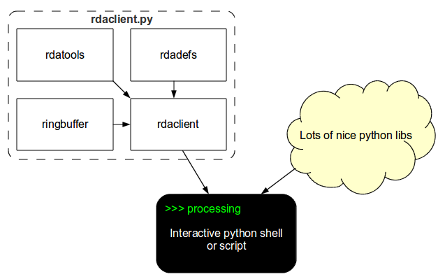
Figure 1. rdaclient.py dependency diagram

Architecture

Two main components of the rdaclient.py are the Client and the Buffer

The Client

The rdaclient.py basically does three things:

• receives the data from the remote RDA data source
• writes the data to a buffer
• provides an API for asynchronous data reading

The data is being received and buffered by a separate process (Streamer), which is started and controlled by the Client instance in the main application code. Both processes access the same memory area through the buffer interface, provided by the ringbuffer module (see The Buffer for implementation details). This architecture is illustrated in figure 2 as a part of a BCI (Brain-Computer Interface) loop

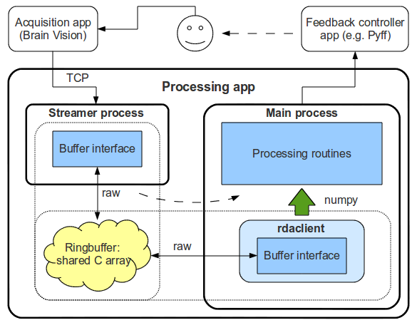
Figure 2. rdaclient.py’s architecture (Processing app)

More information on the interprocess data sharing can be found in the documentation of the python’s multiprocessing package.

The Buffer

ringbuffer is an independent module which was designed to be easily embeddable in python applications which require a contiguous fixed-size ring buffer. It has several important features which make it suitable for the rdaclient.py.

Chunk reading/writing

One of the design goals was to minimize the number of memory copies while reading from the buffer. This is important, for example, when one wants to process the data within a sliding widow and needs to read a large chunk of the same data every time the window is updated.

A usual solution in C will be to return a proper pointer to the processing routine. In python, this is achievable with the help of numpy view objects. The problem, however, arises when the write pointer reaches the end of the array (the buffer is full). Since it’s a ring buffer, the write pointer is set to the beginning of the array to overwrite the old data. Any data chunk that is more than one sample long will now be non-contiguous in memory (split into tail and head parts). This makes it impossible to create a numpy view object and the whole data chunk has to be copied before it’s passed to a processing routine. If the length of the data chunk is known (like in the case of a sliding window reading), it is possible to subdivide the buffer array into two parts: a working array and a pocket. The way this approach works around the aforementioned problem is illustrated in figure 3.

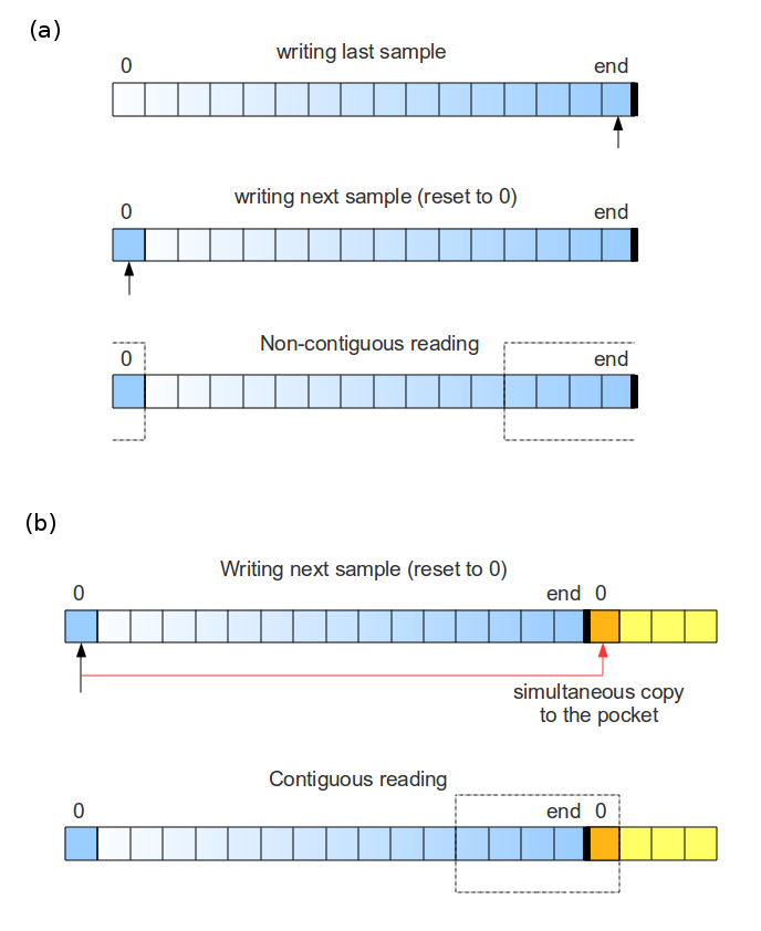
Figure 3. Buffer writing and reading (b) with and (a) without a pocket.

Data and interface separation

The buffer consists of a buffer interface (defined by a RingBuffer class) and the raw sharectypes byte array, which contains both data and the metadata, i.e. all the information about the buffer’s state.

Such interface and data separation makes it possible to use the buffer simultaneously by several processes. The possible algorithm can be:

• A RingBuffer object is created and initialized in one of the processes.
• newly generated raw array is shared between the child processes.
• those processes create their own RingBuffer objects and initialize them from the raw array (initialize_from_raw())provided by the parent, so that they all point to the same shared array.

The raw array has the following structure:

1. The header section:

   Contains the metadata such as size of the sections, current write pointer, datatype, number of channels (number of columns) and total number of samples (not bytes) written

2. The buffer section:

   Contains the actual data in the buffer. When the write pointer reaches the end of the section it jumps to the beginning overwriting the old data. This section is further subdivided into the working and the pocket sections (described above).

Latency

As it was mentioned in previous sections, the rdaclient.py can be used in BCIs. Therefore, it’s very important to have an idea about the latencies appearing when transferring the data along the path Amplifier -> Recording Machine -> Processing machine.

Set up

Unfortunately, it’s pretty hard to measure exactly the Amp -> ... -> Client latencies. Alternatively, one can assemble a closed BCI-like loop and measure the turnover time as the upper bound of the aforementioned latency. The results below are obtained using the system shown in figure 4. A simple algorithm was used to produce a “spike train” which was then recorded and analysed:

1. generate a spike-like signal and send it to the EEG Cap through the audio system
2. listen for the incoming data (from the Amplifier)
3. once the spike is detected, go to 1.

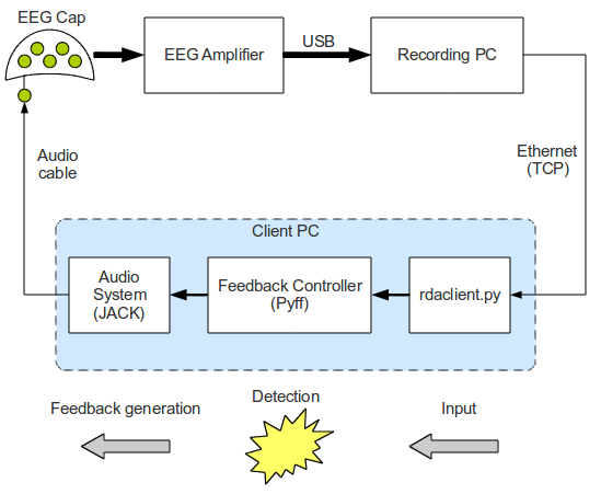
Figure 4. A simple BCI-like loop, used for measuring latencies

The recording machine’s configuration:

• Sampling frequency: 500 Hz
• Block size: 10 samples
• Number of channels: 64
• Theoretical inter-block interval: 20 ms.

The Pyff framework was used for generating the feedback signal and sending it to the audio system through the python interface (pyjack) to the low-latency audio library (JACK). To minimize the latency introduced by the audio buffer, JACK was configured as follows:

• frames per period: 16
• periods per buffer: 2
• sampling rate: 96000

This, in combination with a real-time system kernel, allowed for a theoretical audio latency of 0.333 ms.

Results

The time intervals between the data-block arrivals at the client-side often exceed the theoretical value of 20 ms more than twice (figure 5). Moreover, their distribution has a number of sharp peaks, none of which corresponds to the 20 ms value. Such peaky distribution is most probably caused by a server, since disabling the Nagle’s algorithm (TCP overhead minimization) had no effect.

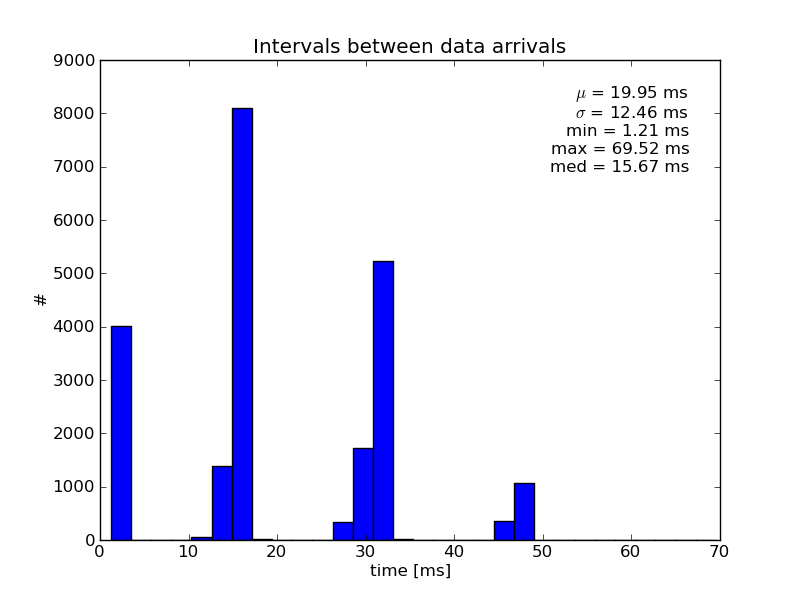
Figure 5. Inter-block intervals at the receiving side

Because the complete loop contains several additional latency sources, the average turnover time was considerably larger (~80 ms) than the average inter-block interval of about 20 ms (figure 6). The potential latency sources are:

• the inter-process communication between the Client and the Feedback Controller
• python interface to JACK
• audio buffer latency (unlikely)
• capacitive effects of the computer-cap connection elements (soldering blobs, clamps, etc.)

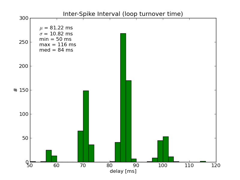
Figure 6. The Generation -> Recording -> Detection -> Generation loop times

Further development

There are some basic features left unimplemented:

• marker handling
• support for different data types (e.g. int16 support)

Marker handling can, for example, be implemented as a static method of the rdadefs.rda_msg_data_t class. Different data types support can be more demanding, since it’ll require several classes and methods to be re-factored.

The control path between the main process and the Streamer is currently implemented rather as a workaround and should probably be redesigned.

Finally, overall stability improvements should be considered.